Representation Learning As A Scientific Key I

One of the challenges of the future will be to make AI/ML more accessible and interpretable for domain experts. The success of the method so far has been the fact that, on the basis of very large data sets, the representations could be chosen by the algorithm, e.g. in a supervised learning process, where the algorithm only takes the data and the target. No matter what we do with Deep Learning, we always have to deal with a certain amount of representation learning, even if it is only with the internal representations within a network, for example.

It has already been empirically shown several times how strongly a machine learning algorithm is based on the selected representations of the data. The most common methods that we have observed in recent years have mainly been concerned with the interpretable domain of natural images (MNIST, ImageNet, etc.). But in my opinion, it will be interesting in those areas where there is a huge amount of data available, but where it can only be partially interpreted reliably by a domain expert. Those data sets are mainly found in areas of the natural sciences. In this short series I’ll talk about Representation and Transfer Learning and a specific example from digital spectral pathology.

What is the idea of Representation Learning?

Actually, this is intuitively simple. Instead of using the entire range of features along the sample space, the algorithm looks for the best representation of the data within that sample space, which can be used to construct better classifiers for example. Further in a different setting it can act as the perfect regularizer for the learning complicated functions. In the last case, my concern will apply.

Why should we care about Rerpesentation Learning?

The core idea is that the network function is some mapping of input to output, in the given form: \f_{Net}(x_{i} = Output_{Net})\). But as an absolutely wonderful example, of which I have unfortunately forgotten where I got it, look at the difference between roman and arabic numerals from figure 1A). Imagine you have a mathematical term consisting of roman numerals. Before you could perform the individual arithmetic steps, you would first have to start by converting the digits into your usual system of representation. Important milestones in the processing of data by Machine Learning were often first related to pre-processing, something that, mind you, is not eliminated by Deep Learning, but transferred in another direction. Especially the domain-related processing cannot be bypassed by representation learning, or the learning time of the network is considerably prolonged under certain circumstances.

I will also discuss other aspects of representation learning in this series, but the first point here relates to a relatively old technique, which is called unsupervised pretraining. This is one of the reasons for the current success of Deep Learning, so to speak. Most of the beginning was dealing with models called Deep Belief Nets 1 or Restricted Boltzmann Machines 2 e.g., but one of the major steps came with the greedy layerwise training and the combination with the Stacked Autoencoder model.3, 4, 4. Goodfellow , Bengio and Courville 5 discuss a a paper from 2015 6, where the authors used unsupervised pretrainig on different data sets and compared their results to a random forest classifier. Overall, it could be seen that the models that worked with unsupervised pretraining performed either slightly worse or much better. Considering this fact, it must be clear that the question, i.e. the data set, decides when one should use unsupervised pretraining. Before we go into the details of unsupervised pretraining, let’s ask ourselves (and this paper 7) what makes a good representation. The perfect representation can be considered as a particular from of a prior assumption, which Erhan et al. call “data-dependent prior on the parameters”. This concept can include the following ideas

• This prior is able to smooth the learning function of: \f_{Net}(x_{i} = Output_{Net})\
• This prior is capable of combining or disentangle multiple explanations of the data generation process. (In particular, this point will later become important for the example presented.)
• This prior is capable of strengthing the shared factors of multiple models (I’ll show you this later, when we Talk about Transfer-Learning)
• This prior can act as a form of data-dependent regularizer

The last point will become quite important, because measured data in scientific settings is quite different to the most audio and visual data that you are processig every day, as I’m going to show you in this series.

Unsupervised Pretraining and Fine-Tuning

This method is primarily based on the question of how deep neural networks can and should be initialised. In this method, the weights from the unsupervised pre-training are taken as starting values for the so-called fine-tuning. Later in the series I will try to refer to these parameters and take a closer look at them. But first of all, what is exactly unsupervised learning and the transfer learning behind it. If you look at figure 1B) you will see a clear simplification of a figure from the Bengio et al. paper 7 on representation learning. Here we can see how learned parameters from unsupervised pretraining can be used as a basis for further models. Methodologically, I refer here mainly to the stacking of autoencoders and the procedure known as greedy layer-wise training. Further, I will try to summarise the Bengio paper and parts of the Deep Learning book 5 here.

First of all, what exactly is the greedy-layer-wise method and why can it be useful in processing scientific data? In figure 1C) you see basically the idea behind the manifold interpretation of this procedure. In short, you see that when you train with corrupted input signal this training procedure is able to recover the underlying structure of the data generating manifold. You see the line which represents the given manifold, while the stars representing the data lying on this manifold. The red dots are standing for the corrupted input data and by looking at the direction of the arrows, you see what ths training procedure basicalyy does. While recovering the stars from the red dots the model learns specific data-relevant representations, that we’re interessted in. If your thinking in terms of code, this greedy-layer-wise method of training those stacked autoencoders is pretty simple. You basically have one Autoencoder at every training stage. I won’t go into the specific details of the Autoencoder model, but you should know it, because it is somehow present in every modern learning model of the so called latent varaiable or generative models. By the way it is present for a very long time at the machine learning landscape. Chris Bishops great Book on “Neural Networks in Pattern Recognition” 8 gives credits to Bourlard/Kamp (1988) 9 and Baldi/Hornik(1989), while these authors 5 give the credits to LeCun (1987) adn his PhD Thesis. It doesn’t really matter, but these autoassociative models have been around for quite a long time. The specfic idea I’m talking about is based on the following two references, especially the second 10, 11.

It addresses directly the idea of Fig 1C) (this is where got it from! 10). In order to get useful representations you have to regularise the learning of the model (AE).

Not the Conclusion

Actually this we’ll be rather long series so before explan the model in source code, which is quite simple, I will explain the data that I used.

Spectroscopic data are well known to those who work with me, but if I’m going to put it on the net, I should also explain in general why the data were so difficult to process, that I come back to the unsupervised pretraining here. So next stop we’ll be post about the data.

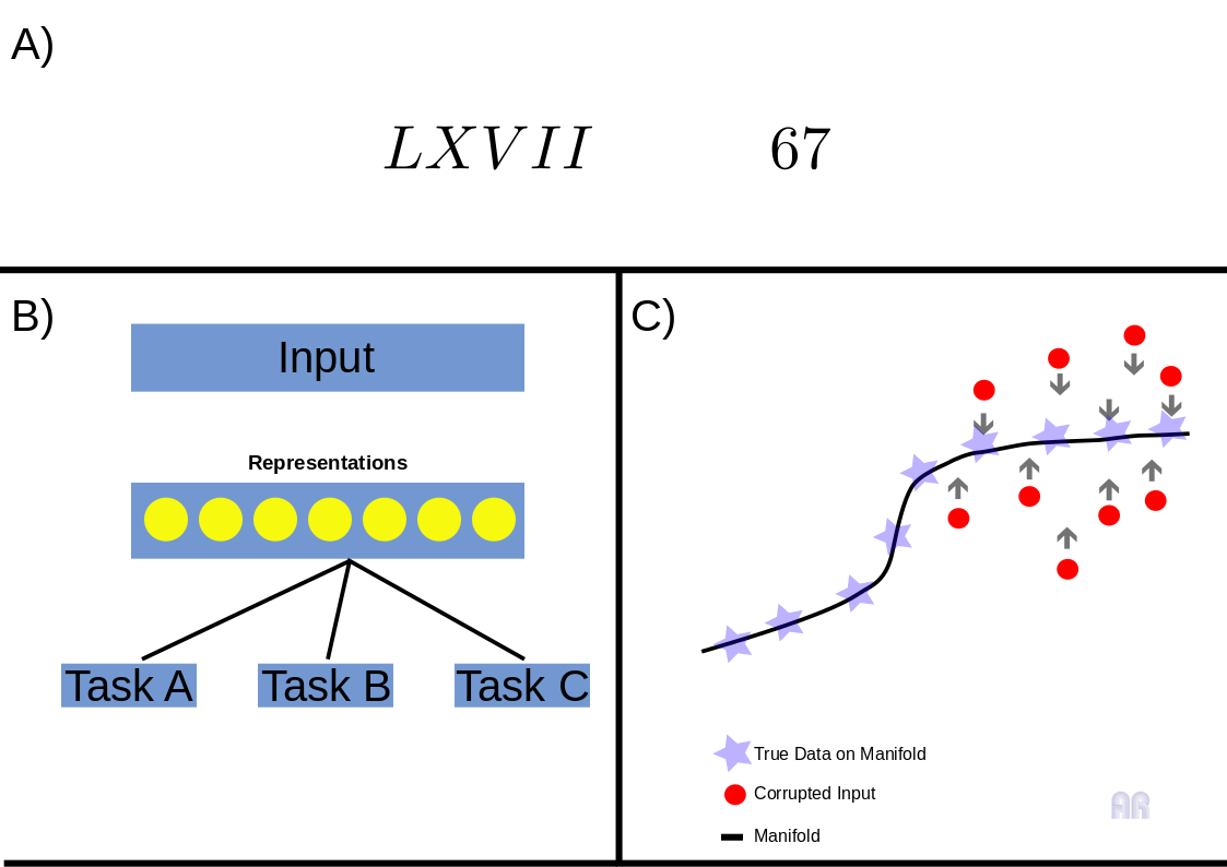Fig.1