The World Does Not Only Consist Of MNIST Data I

In the field of empirical data it often happens that the measurements contain errors. In the case of a learning algorithm, such as deep neural networks, it can happen that no generalization is desired in the case of a model.

In almost all cases in the empirical sciences, the target variable is more a summary or abstraction. The comparison to MMIST shows that a 28x28 matrix with values between 0 and 255 is interpretable for us at any time, if we use the correct graphical representation in form of a picture. But if we measure a physical quantity and connect it to a basic hypothesis as a target variable, it can be quite difficult to teach it to a model or algorithm.

A First Model

My experience shows that in most cases the physical measurements are less accurate than assumed by the test person, or the data set is very small and has a very high noise level. This whole point, leads you to assume at the beginning, that the whole training data set will not contain any false positives or negatives, just because the domain expert assures you and he will assure you that you should not doubt his competence. ;) So, if you run into problems, in most cases you will have to reverse engineer the training data set and discuss this with the domain expert.

One point which almost always makes the start, is a first, mostly over-adapted, model to the data. Here two things have to be separated, the training error \(Err_{\tau}\) and the training loss \(\mathcal{L} (Y, f(X))\). I have seen the former converge to a very passable value in many models, the latter is more meaningful in a different sense. Within the framework of gradient based models, like DNNs, the parameters are adjusted to best explain the training data set. This procedure is done in the context of mathematical optimization along the gradients.

Here is an example, I trained a small CNN on CT data of the lung to be able to make a medical diagnosis at the end. From the references below you can see the underlying paper and the data itself. For my test here I used and splitted only the training data. Furthermore, I made two changes to the target variable of my training data set:

• 1) 5% of the labels were randomly changed
• 2) 10% of the label were randomly changed.

In both cases the test data set remained unchanged and the same hyper-parameters and seeds were used for all of the three models.

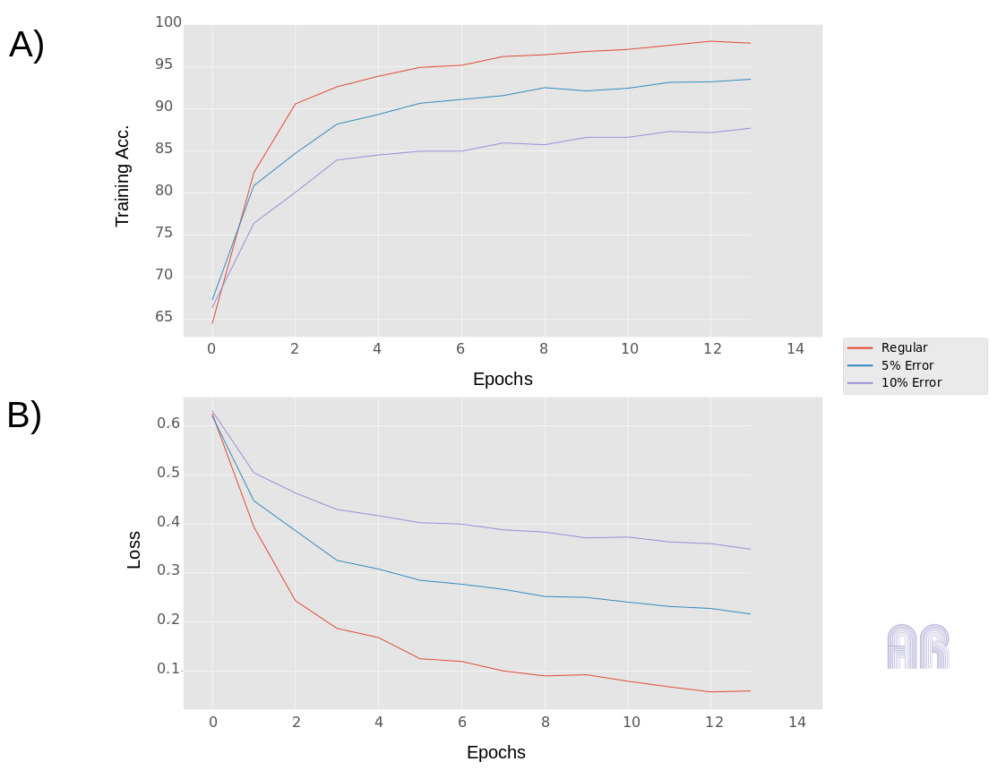Fig.1

The first figure shows, how training errors and loss behave on the same data set using different errors on the target. The red curve shows the regular course without artificial errors, the blue curve shows the course using a 5% error in the training data set and the purple curve shows the whole for a 10% error. I’m not going to make the point here, that an target error can be estimated directly from the curves behavior, but if you look at the slope of the loss curves, you can easily see how it changes. So keep that in mind! The model I have chosen is deliberately small and should have quickly exhausted its capacities and run into overfitting, so training errors converge!

At this point I would suggest to use exactly this idea, add noise to the target variable, for example 5 and 10% noise and see where your original model lies in comparison of loss curves. This point becomes important when you actually make the network converge over longer period of epochs. As a comparison in Fig.2, here one can see the same networks without known error (regular) in the target variable and with a known 10% error in the target variable.

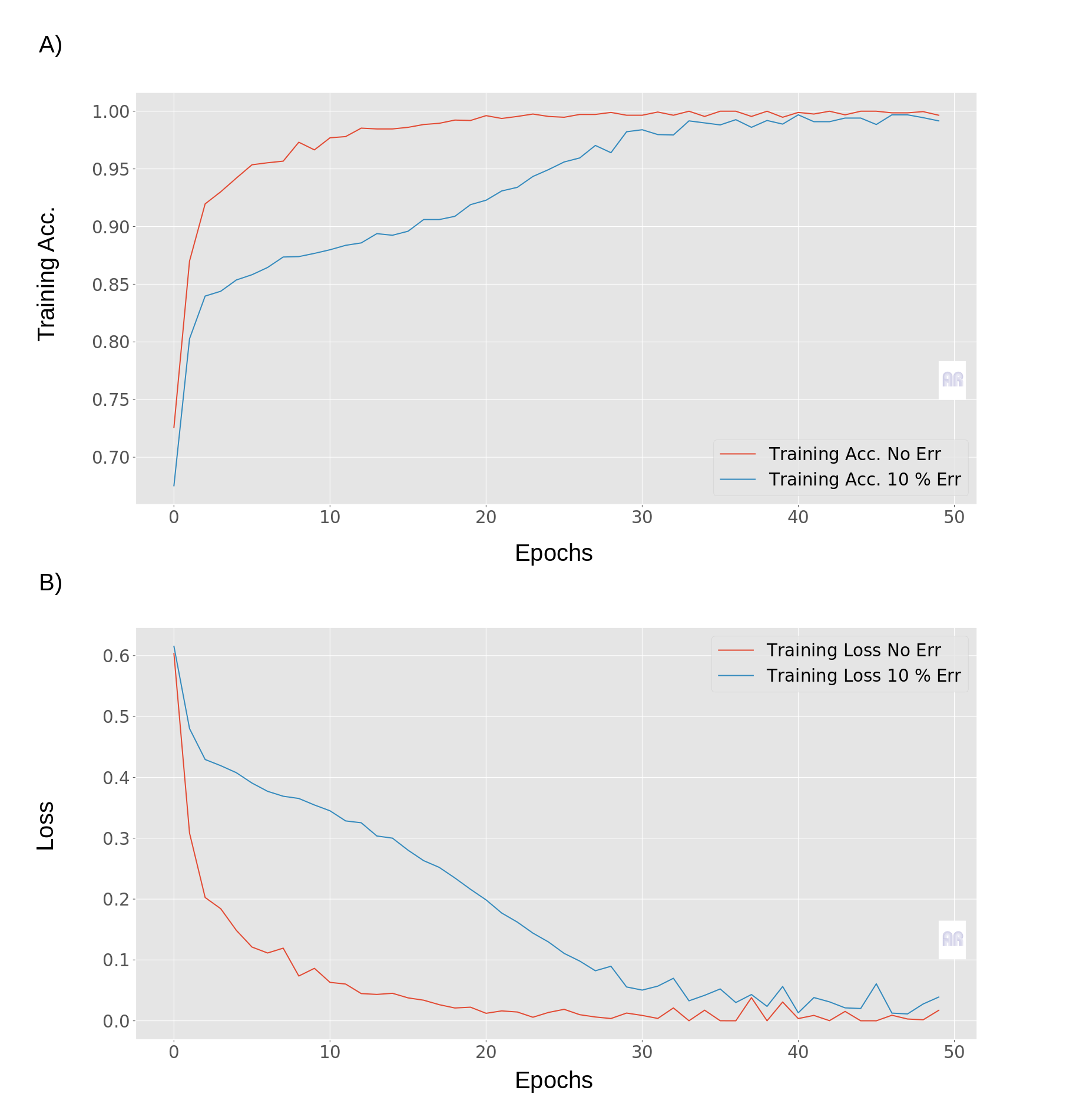Fig.2

If you look at the blue and red curve, the other behaviour is clearly noticeable. What we see is a lower convergence and a clearly different Lipschitz constant of the curves with a 10% error. The red curves for example, show a clear convergence against the min. and max. values of the respective functions.

Experiments

The data that I used for all the experiments in this post, can be found in this Cell paper 1 and in the corresponding online resources of this paper,2. As one can see from the mendeley data-site, it is under the CC 4.0 licence, so I can redistribute it. Important to note, I only used a subset of the data for the experiments!

The implementation for the network was done in Python 3.5 using Keras(2.X) and Tensorflow (1.X).

from sklearn.model_selection import train_test_split
import keras
from keras.datasets import mnist                           
from keras.utils import to_categorical     
import matplotlib.pyplot as plt                            
import numpy as np
from skimage.transform import resize
plt.style.use('ggplot')
import h5py

import keras
from keras.datasets import mnist                                                                                  
from keras.utils import to_categorical     
import matplotlib.pyplot as plt                                 
import numpy as np
def simple_cnn(trX,trY, teX, teY):
  from keras import layers                                                                                        
  from keras import models                      
                                              
  model = models.Sequential()                                                 
  model.add(layers.Conv2D(32, (3, 3), activation='relu', input_shape=(64, 64, 1)))
  model.add(layers.MaxPooling2D((2, 2)))                 
  model.add(layers.Conv2D(64, (3, 3), activation='relu'))
  model.add(layers.MaxPooling2D((2, 2)))
  model.add(layers.Conv2D(64, (3, 3), activation='relu'))
  model.add(layers.Flatten())                      
  model.add(layers.Dense(64, activation='relu'))
  model.add(layers.Dense(2, activation='softmax'))
                                                  
  model.compile(optimizer='rmsprop',                                                                              
                loss='categorical_crossentropy',
                metrics=['accuracy'])         
  history = model.fit(trX,trY, epochs=150, batch_size=64)
  test_loss, test_acc = model.evaluate(teX, teY)
  print("Test Loss",test_loss) 
  print("Test Acc",test_acc) 
  return(history,model ,test_acc)

Conclusion

I think that in a gradient based learning, the algorithms give a lot of possibilities to see such learning curves (hyperparameters), but my experience also tells me, that the inspection of such a learning curve is always worth to take a closer look at the data. In the course of the optimization, there should always be an overadaptation/overfitting to the training data set, if there is no regularization outside the inherent, such as convolution layers.

Based on the model above, one can easily imagine how overfitting can occur here. This model offers, with two convolutional layers and one dense layer, only little capacities and therefore runs fast into the overfitting of the training data set! This is almost always my first workflow point, in problems that have to do with simple classification like this.