Model Assesment and Ensemble Techniques I

What Is Generalization ?

Most of the models that have a direct application in current research in the natural sciences can be said to be roughly divided into two areas. The first part is largely based on the classifiers and the second part on the generative models. However, all these models have one thing in common, the question of how well they can actually provide robust answers or how well they can generalize. I have seen many simple applications fail exactly at this point, and therefore I try to bundle some resources here.

When evaluating a model, certain parameters are considered which can provide information about its performance. The actual performance level of all models is measured by how well unknown data can be processed by such a model, and how far the prediction is away from the ground truth.

Mathematical Description

Something we want to look at directly in the performance analysis is the so-called generalization error of a model. This is defined as follows: \[ Err_{\tau} = E[\mathcal{L} (Y, f(X)) | T ] \]

For a better explanation of the above formula, the individual components must be explained:

We have a data set which consists of a set of vectors \(X_{i}\). Furthermore, in the context of supervised learning, we also have a target value for each input vector \(Y_{i}\). The model we have, symbolizes itself as a function in form of \(f(X) = \hat{Y}\), which returns a prediction in the form of \(\hat{Y}\) to an input vector \(X\). The difference between the target value \(Y\) and the output of the model \(\hat{Y}\) is considered by the loss function \(\mathcal{L} (Y, f(X))\). The above definition refers exclusively to the generalization error \(Err_{\tau}\) when using the training set \(\tau \). But what we actually want to have is the generalization of this value to an independent test set. Apart from the generalization to the test set, most methods, which I will discuss later, give the expected value in the form of: \[ Err = E[\mathcal{L} (Y, f(X))] = E[Err_{\tau}] \] So, to get an estimate in the form of \(Err\), there are roughly two possible ways you can take.

• The estimation via an analytical procedure in the form of methods like the AIC or the BIC.
• Estimation through modelling and reuse of training data as a sampling procedure as in Cross-Validation and the bootstrap method.

Since this is the most common method, I will start with the idea of cross-validation. To do this, we need to agree on a procedure and nomenclature for data splitting. I actually always used the one from ELSII (Hastie,Tibshirani,Friedman). With a sufficent amount of data, you can split your complete data-set into three distinct parts (Fig.1). The Training part (\(\tau \)), which we’ll use for the fitting of the model to the data. The second part is the so called Validation-Data, which you need to keep track on the overfitting of the training process and the last one is called the Test-data. Test-data is used to get an estimate of the \(E[Err_{\tau}] \)

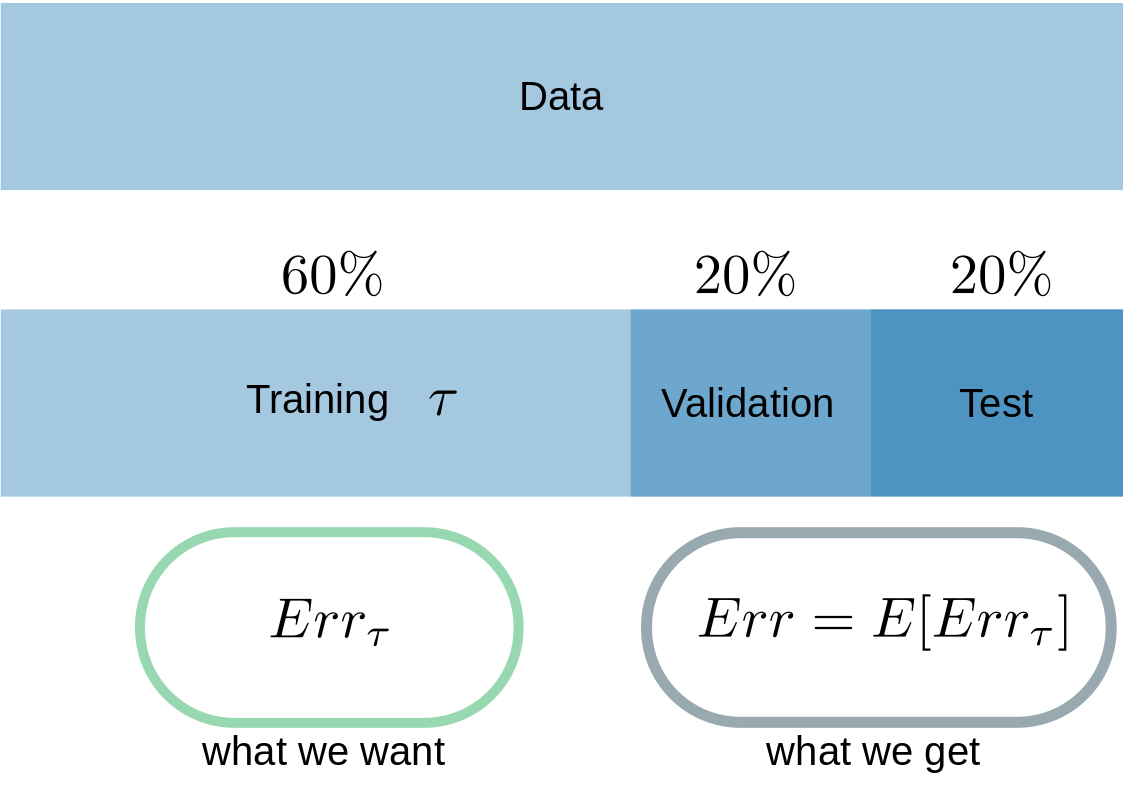Fig.1

As far as I can see from the literature, there’re a tons of rule of thumbs on how to devide the data, but I use this one from Fig.1 and it worked for me so far.

\(\) \(\) But for now to the first method of cross-validation. The basic idea of the cross validation is based on multiple sampling of the data set without replacement.

\[ CV(f(X)) = \frac{1}{N} \sum_{i=1}^{N} \mathcal{L} (Y_{i}, f^{-k(i)}(X_{i })) \]

from sklearn.model_selection import train_test_split
import keras
from keras.datasets import mnist                                                                                       
from keras.utils import to_categorical     
import matplotlib.pyplot as plt                                 
import numpy as np

def simple_cnn(trX,trY, teX, teY):
  from keras import layers                                                                                               
  from keras import models                      
                                              
  model = models.Sequential()                                                 
  model.add(layers.Conv2D(32, (3, 3), activation='relu', input_shape=(28, 28, 1)))
  model.add(layers.MaxPooling2D((2, 2)))                 
  model.add(layers.Conv2D(64, (3, 3), activation='relu'))
  model.add(layers.MaxPooling2D((2, 2)))
  model.add(layers.Conv2D(64, (3, 3), activation='relu'))
  model.add(layers.Flatten())                      
  model.add(layers.Dense(64, activation='relu'))
  model.add(layers.Dense(10, activation='softmax'))
                                                  
  model.compile(optimizer='rmsprop',                                                                                     
                loss='categorical_crossentropy',
                metrics=['accuracy'])         
  history = model.fit(trX,trY, epochs=5, batch_size=64)

  test_loss, test_acc = model.evaluate(teX, teY)

  print("Test Loss",test_loss) 
  print("Test Acc",test_acc) 

  return(history,model ,test_acc)

The first code section shows a very simple CNN in the Keras/TF API. The model itself is rather unimportant at this point, because I just tried to concentrate on the process of validation by CV.

def do_cv(folds):
  (train_images, train_labels), (test_images, test_labels) 
  = mnist.load_data()
                                                                                  
  train_images = train_images.reshape((60000, 28, 28, 1))
  train_images = train_images.astype('float32') / 255    
                                        
  test_images = test_images.reshape((10000, 28, 28, 1))  
  test_images = test_images.astype('float32') / 255
                                                
  train_labels = to_categorical(train_labels)      
  test_labels = to_categorical(test_labels)

  numv_samples  = int(len(train_images) / folds)
  #Fs = []

  errs_ = []
  mods_ = []
  hists_ = []
  #print(numv_samples.shape)
  for i in range(folds):
    print("Folds", i)
    
    valdat = train_images[i * numv_samples: (i + 1) * numv_samples]
    
    print(valdat.shape)
    
    valtarget = train_labels[i * numv_samples: (i + 1) * numv_samples]
    
    print(valdat.shape)

    ktrdat = np.concatenate([train_images[:i * numv_samples], 
      train_images[(i + 1) * numv_samples:] ], axis=0 )
    print(ktrdat.shape)
    ktrtarget = np.concatenate([train_labels[:i * numv_samples], 
      train_labels[(i + 1) * numv_samples:] ], axis=0 )
    print(ktrtarget.shape)
    #Fs.append([ktrdat, ktrtarget ,valdat, valtarget ])
    history,model,test_acc = simple_cnn(ktrdat,ktrtarget, valdat, valtarget)
    errs_.append(test_acc)
    hists_.append(history)
    mods_.append(model)
  en = np.array(errs_)
  print("Average Error in Cross-Validation", en.mean())
  return hists_,mods_,errs_

The second code section shows exactly that part of the actual cross-validation, which is based on the fact that there is no replacement, but closed areas between training and validation data per fold. This is exactly the point where there is a clear demarcation to the bootstrap, because there is the sampling done with replacement, which makes this method showing more over-adapted values for the generalization error than the CV. But I will come to the bootstrap later.

def box(e):
  plt.rcParams.update({'font.size': 22})
  green_diamond = dict(markerfacecolor='g', marker='D')
  fig1, ax1 = plt.subplots()
  ax1.set_title('Box-Plot')
  plt.ylabel('Test-Acc. in %')
  ax1.boxplot(e,flierprops=green_diamond)
  plt.show()
  return

The third code block shows only a plot command for creating boxplots of the individual error portions per fold. Here, after the model has been fiited against the individual data in the folds, the graphical evaluation of the error terms and their inter-quartiles can be generated.

As can be seen from Figure 2, there are sometimes significant differences in the interquartiles for the boxplots generated in this way. This variance is based on the number of data points but not directly on the number of folds. Figure 2 A) shows a 5 fold CV and B) shows 10-fold CV on the same dataset. 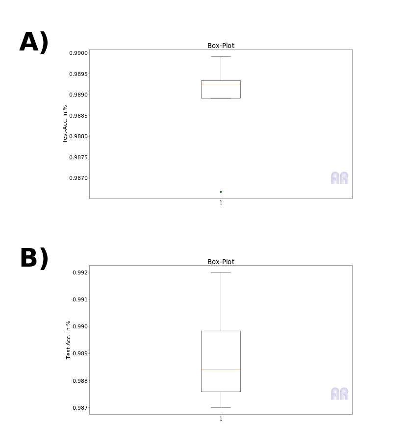Fig.2: A) 5-Fold, B) 10-Fold

Conclusion

The pure cross-validation is certainly not the last word of wisdom, but it is good estimator, and it is less prone to overfit than the (pure) bootstrap method. The variance between the folds is based on the fact that for N small data sets, the similarity increases below the folds. So if I take too few folds with too little data, this variance increases. A successful remedy for this is the idea of the leave-one-out CV. With this modification on the value for K = N is set and the similarity of the different datasets reduces the variance. Now let’s imagine here a learning method like a deep neural network, if we set K = N, the training takes forever and eats enormous resources.

This would be impractical in itself, because what we want is an estimate and actually a statement about whether the model predicts particularly well on a certain range of training/test set without being able to generalize. This point is also clear with a 5 Fold CV, but it should be noted that the number of training points N is decisive. In fig. 2 I trained against the pure test set of the MNIST database and even split these 10k points into 80%/20% folds.

References

The Elements of Statistical Learning 1

Symonds and Moussalli, 2011 2

Introduction To Data Mining 3